Sparse arrays and the CESM land model component#
An underappreciated feature of Xarray + Dask is the ability to plug in different array types. Usually we work with Xarray wrapping a Dask array which in turn uses NumPy arrays for each block; or just Xarray wrapping NumPy arrays directly. NumPy arrays are dense in-memory arrays. Other array types exist:
Over the past few years, significant effort has been made to make these array types speak a common protocol so that higher-level packages like Xarray can easily wrap all of them. The latest (and hopefully last) version of these efforts is described at data-apis if you are interested.
This notebook explores using sparse arrays with dask and xarray motivated by some Zulip conversations around representing “Plant Functional Types” from the land model component. A preliminary version of this notebook is here; and the work builds on PFT-Gridding.ipynb
Importing Libraries#
%matplotlib inline

import cartopy.crs as ccrs
import matplotlib as mpl
import matplotlib.pyplot as plt
import numpy as np
import sparse
import xarray as xr

# some nice plotting settings
xr.set_options(cmap_sequential=mpl.cm.YlGn, keep_attrs=True)
plt.rcParams["figure.dpi"] = 120
cbar_kwargs = {"orientation": "horizontal", "shrink": 0.8, "aspect": 30}


def setup_axes():
    ax = plt.axes(projection=ccrs.PlateCarree())
    ax.coastlines()
    return ax
Community Land Model (CLM) output#
Lets read a dataset.
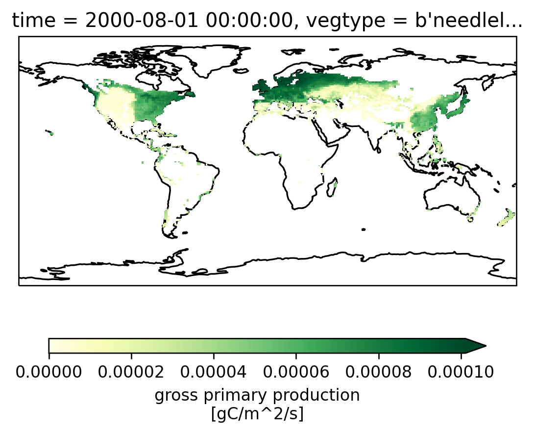
This dataset represents monthly mean output from the Community Land Model (CLM), the land model component of CESM. The particular variable here is gross primary production (GPP), which is essentially photosynthesis or carbon uptake by plants. Because CLM represents different plant functional types (PFTs) within a single model grid cell (up to 79 different types including natural vegetation and crops), this dataset includes information on how GPP varies by PFT. This way we can examine photosynthesis and how it varies across different plant types. To visualize this output, we often need to remap the information to a latitude/longitude grid, preserving plant type.
pft_constants = xr.open_dataset(
    "/glade/p/cesm/cseg/inputdata/lnd/clm2/paramdata/clm5_params.c190529.nc"
)
pftnames = pft_constants.pftname
data = xr.open_dataset(
    "/glade/p/cgd/tss/people/dll/TRENDY2019_History/S0_control/TRENDY2019_S0_control_v2.clm2.h1.GPP.170001-201812.nc",
    decode_times=True,
    chunks={"time": 100},
)
data
<xarray.Dataset>
Dimensions:             (levgrnd: 25, levlak: 10, levdcmp: 25, lon: 288, lat: 192, gridcell: 21013, landunit: 48359, column: 111429, pft: 166408, time: 3828, hist_interval: 2)
Coordinates:
  * levgrnd             (levgrnd) float32 0.01 0.04 0.09 ... 19.48 28.87 42.0
  * levlak              (levlak) float32 0.05 0.6 2.1 4.6 ... 25.6 34.33 44.78
  * levdcmp             (levdcmp) float32 0.01 0.04 0.09 ... 19.48 28.87 42.0
  * lon                 (lon) float32 0.0 1.25 2.5 3.75 ... 356.2 357.5 358.8
  * lat                 (lat) float32 -90.0 -89.06 -88.12 ... 88.12 89.06 90.0
  * time                (time) object 1700-02-01 00:00:00 ... 2019-01-01 00:0...
Dimensions without coordinates: gridcell, landunit, column, pft, hist_interval
Data variables: (12/51)
    area                (lat, lon) float32 dask.array<chunksize=(192, 288), meta=np.ndarray>
    landfrac            (lat, lon) float32 dask.array<chunksize=(192, 288), meta=np.ndarray>
    landmask            (lat, lon) float64 dask.array<chunksize=(192, 288), meta=np.ndarray>
    pftmask             (lat, lon) float64 dask.array<chunksize=(192, 288), meta=np.ndarray>
    nbedrock            (lat, lon) float64 dask.array<chunksize=(192, 288), meta=np.ndarray>
    grid1d_lon          (gridcell) float64 dask.array<chunksize=(21013,), meta=np.ndarray>
    ...                  ...
    mscur               (time) float64 dask.array<chunksize=(100,), meta=np.ndarray>
    nstep               (time) float64 dask.array<chunksize=(100,), meta=np.ndarray>
    time_bounds         (time, hist_interval) object dask.array<chunksize=(100, 2), meta=np.ndarray>
    date_written        (time) object dask.array<chunksize=(100,), meta=np.ndarray>
    time_written        (time) object dask.array<chunksize=(100,), meta=np.ndarray>
    GPP                 (time, pft) float32 dask.array<chunksize=(100, 166408), meta=np.ndarray>
Attributes: (12/102)
    title:                                     CLM History file information
    comment:                                   NOTE: None of the variables ar...
    Conventions:                               CF-1.0
    history:                                   created on 09/27/19 16:25:57
    source:                                    Community Terrestrial Systems ...
    hostname:                                  cheyenne
    ...                                        ...
    cft_irrigated_tropical_corn:               62
    cft_tropical_soybean:                      63
    cft_irrigated_tropical_soybean:            64
    time_period_freq:                          month_1
    Time_constant_3Dvars_filename:             ./TRENDY2019_S0_constant_v2.cl...
Time_constant_3Dvars: ZSOI:DZSOI:WATSAT:SUCSAT:BSW:H...The GPP DataArray has 2 dimensions: time and pft where pft is really a compressed dimension representing 3 more dimensions in the data (lon, lat, and vegtype of sizes 288, 192, and 79 respectively). Each index along the pft dimension represents a single point in (vegtype, lat, lon) space and only (lat, lon) points corresponding to land cells are saved.
This output is naturally sparse (no trees on the ocean surface 😆), so we’ll explore using spare arrays to represent the data
data.GPP
<xarray.DataArray 'GPP' (time: 3828, pft: 166408)>
dask.array<open_dataset-e503263520abd161067be1f5e311c2e1GPP, shape=(3828, 166408), dtype=float32, chunksize=(100, 166408), chunktype=numpy.ndarray>
Coordinates:
  * time     (time) object 1700-02-01 00:00:00 ... 2019-01-01 00:00:00
Dimensions without coordinates: pft
Attributes:
    long_name:     gross primary production
    units:         gC/m^2/s
cell_methods: time: meanGoal#
Our goal here is to expand this 2D GPP dataarray to a 4D sparse array (time, type, lat, lon).
This way no extra memory is used to represent NaNs over the ocean.
We get to work with a substantially simpler representation of the dataset.
We develop the following two functions: to_sparse and convert_pft_variables_to_sparse (presented in the hidden cell below)
Now we run one of the developed functions to convert pft variables to sparse
sparse_data = convert_pft_variables_to_sparse(data, pftnames)
sparse_data.GPP
<xarray.DataArray 'GPP' (time: 3828, vegtype: 79, lat: 192, lon: 288)>
dask.array<transpose, shape=(3828, 79, 192, 288), dtype=float32, chunksize=(100, 79, 192, 288), chunktype=sparse.COO>
Coordinates:
  * lat      (lat) float64 -90.0 -89.06 -88.12 -87.17 ... 87.17 88.12 89.06 90.0
  * lon      (lon) float64 0.0 1.25 2.5 3.75 5.0 ... 355.0 356.2 357.5 358.8
  * time     (time) object 1700-02-01 00:00:00 ... 2019-01-01 00:00:00
  * vegtype  (vegtype) |S40 b'not_vegetated                           ' ... b...
Attributes:
    long_name:     gross primary production
    units:         gC/m^2/s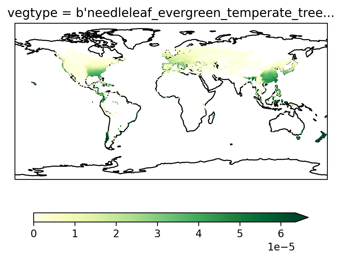
cell_methods: time: meanEasy visualization#
Once converted to a 4D sparse array, visualization of the dataset is now easy
ax = setup_axes()
sparse_data.GPP.isel(vegtype=1, time=3606).plot(robust=True, ax=ax, cbar_kwargs=cbar_kwargs)
<cartopy.mpl.geocollection.GeoQuadMesh at 0x2ae53f25af40>
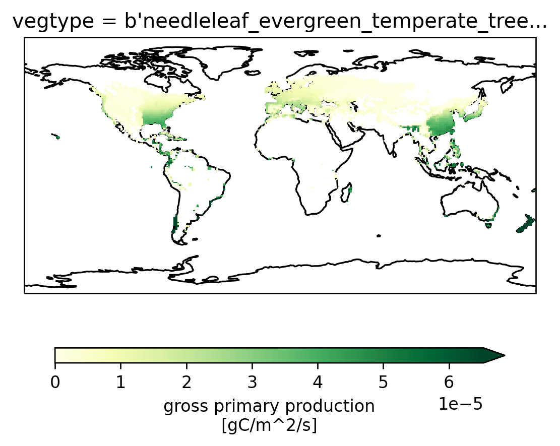
Many xarray operations just work#
Here’s a monthly climatology for January (calculated using the first two years only to reduce computation time).
ax = setup_axes()
(
    sparse_data.GPP.isel(vegtype=1, time=slice(24))
    .groupby("time.month")
    .mean()
    .sel(month=1)
    .plot(robust=True, ax=ax, cbar_kwargs=cbar_kwargs)
)
<cartopy.mpl.geocollection.GeoQuadMesh at 0x2ae53fedf640>
Introduction to sparse arrays#
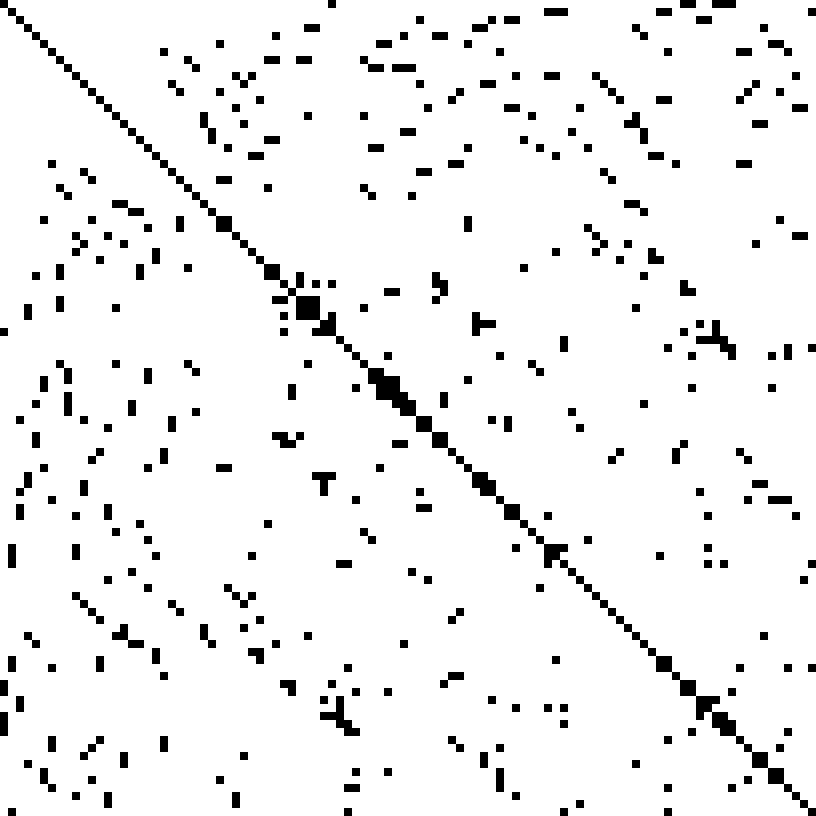
What is a sparse array?#
A sparse array is a n-dimensional generalization of a sparse matrix which is one where most elements are 0 (or some other “fill value”). Significant memory savings are possible by only storing non-zero values and the locations of the those values. A “dense” representation, for example using NumPy, which uses memory for every 0 would use substantially more memory
Here is a visualization from the Wikipedia article where black squares are non-zero.
Constructing a sparse array#
https://sparse.pydata.org/ provides a number of sparse array formats. Here we work with sparse.COO.
We construct a sparse.COO array by passing a list of non-zero data values and the coordinate locations for those values
# in this case shape=(3,3), dtype=np.int64, and fill_value=0 are set by default
eye = sparse.COO(coords=[[0, 1, 2], [0, 1, 2]], data=[1, 1, 1])
eye
| Format | coo |
|---|---|
| Data Type | int64 |
| Shape | (3, 3) |
| nnz | 3 |
| Density | 0.3333333333333333 |
| Read-only | True |
| Size | 72 |
| Storage ratio | 1.0 |
To convert to a dense NumPy array use .todense
eye.todense() # identity matrix!
array([[1, 0, 0],
       [0, 1, 0],
       [0, 0, 1]])
A slightly more complicated example, with a bigger shape, and a custom fill_value
array = sparse.COO(
    coords=[[0, 1, 2], [0, 1, 2]],
    data=np.array([1, 1, 1], dtype=np.float32),
    shape=(4, 4),
    fill_value=np.nan,
)
array
| Format | coo |
|---|---|
| Data Type | float32 |
| Shape | (4, 4) |
| nnz | 3 |
| Density | 0.1875 |
| Read-only | True |
| Size | 60 |
| Storage ratio | 0.9 |
array.todense()
array([[ 1., nan, nan, nan],
       [nan,  1., nan, nan],
       [nan, nan,  1., nan],
       [nan, nan, nan, nan]], dtype=float32)
Sparse arrays with dask#
The idea here is that each dask block is a sparse array (compare the more common case where each block is a NumPy array). This works well, dask recognizes that the chunks are sparse arrays (see Type under Chunk)
import dask.array

dasky_array = dask.array.from_array(array, chunks=2)
dasky_array
|
Wrapping sparse arrays in xarray#
works by passing the sparse array to xarray.DataArray
da = xr.DataArray(array, coords={"x": np.arange(4), "y": np.arange(4)})
da
<xarray.DataArray (x: 4, y: 4)>
<COO: shape=(4, 4), dtype=float32, nnz=3, fill_value=nan>
Coordinates:
  * x        (x) int64 0 1 2 3
  * y        (y) int64 0 1 2 3
Access the underlying sparse array using DataArray.data
da.data
| Format | coo |
|---|---|
| Data Type | float32 |
| Shape | (4, 4) |
| nnz | 3 |
| Density | 0.1875 |
| Read-only | True |
| Size | 60 |
| Storage ratio | 0.9 |
Convert to NumPy using DataArray.as_numpy
da.as_numpy()
<xarray.DataArray (x: 4, y: 4)>
array([[ 1., nan, nan, nan],
       [nan,  1., nan, nan],
       [nan, nan,  1., nan],
       [nan, nan, nan, nan]], dtype=float32)
Coordinates:
  * x        (x) int64 0 1 2 3
* y (y) int64 0 1 2 3Convert and extract the numpy array using DataArray.to_numpy
da.to_numpy()
array([[ 1., nan, nan, nan],
       [nan,  1., nan, nan],
       [nan, nan,  1., nan],
       [nan, nan, nan, nan]], dtype=float32)
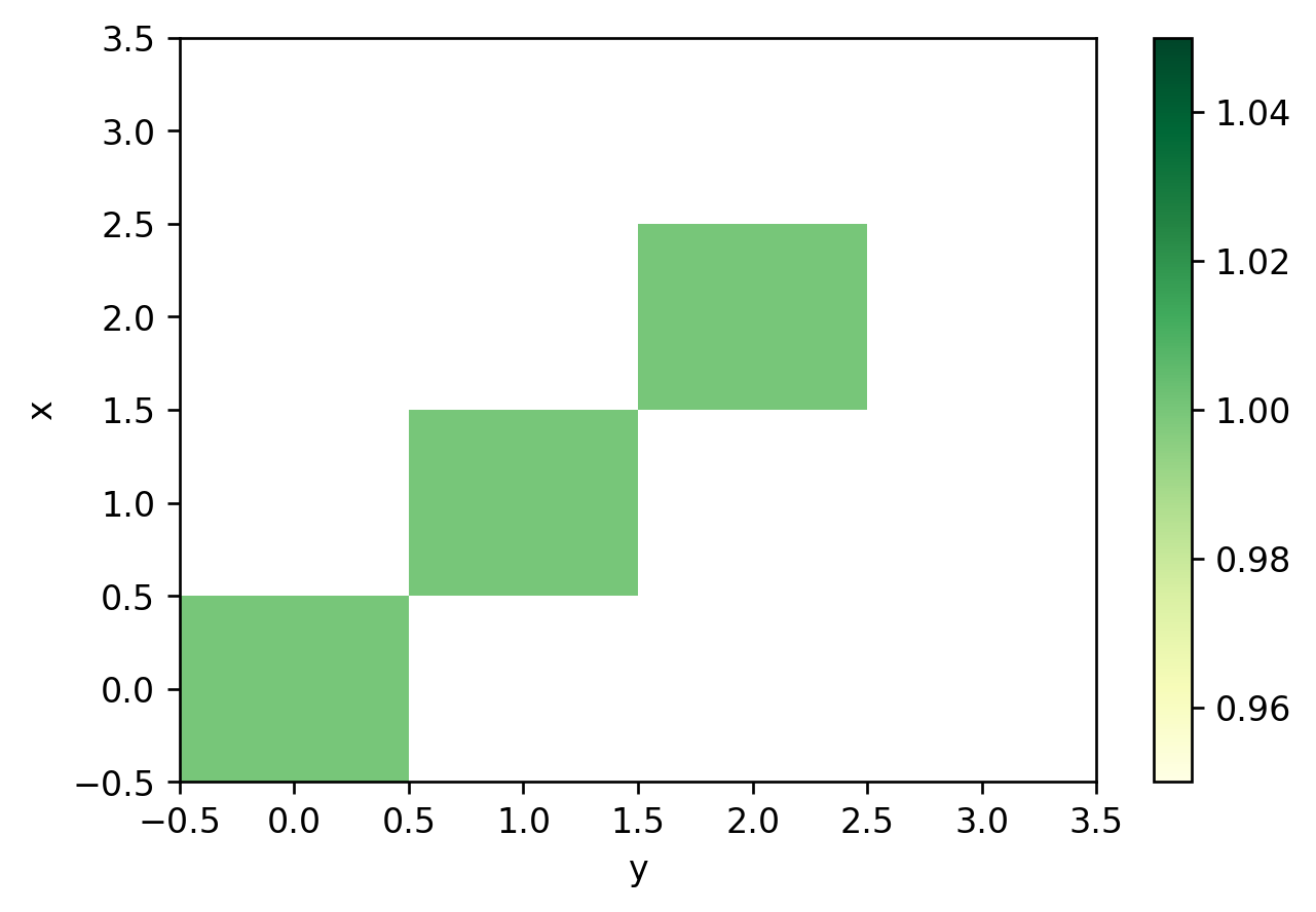
Plotting works easily (the array is “densified”, or converted to a NumPy array, automatically before being passed to matplotlib)
da.plot()
<matplotlib.collections.QuadMesh at 0x2ae53fb0d7f0>
This works.
da.mean("x")
<xarray.DataArray (y: 4)>
<COO: shape=(4,), dtype=float64, nnz=3, fill_value=nan>
Coordinates:
  * y        (y) int64 0 1 2 3
Sparse arrays with dask + xarray#
Xarray knows how to handle dask arrays, so we can just pass dasky_array and things work
xr.DataArray(dasky_array, coords={"x": [1, 2, 3, 4], "y": [1, 2, 3, 4]})
<xarray.DataArray 'array-8e28f4e6653ecaa445c49b8638c8f808' (x: 4, y: 4)>
dask.array<array, shape=(4, 4), dtype=float32, chunksize=(2, 2), chunktype=sparse.COO>
Coordinates:
  * x        (x) int64 1 2 3 4
  * y        (y) int64 1 2 3 4
Back to CLM output#
Convert a single timestep to sparse#
Lets begin with a simple subset of the problem: a single timestep as a numpy array.
subset = data.GPP.isel(time=0).load()
subset
<xarray.DataArray 'GPP' (pft: 166408)>
array([0., 0., 0., ..., 0., 0., 0.], dtype=float32)
Coordinates:
    time     object 1700-02-01 00:00:00
Dimensions without coordinates: pft
Attributes:
    long_name:     gross primary production
    units:         gC/m^2/s
cell_methods: time: meanRecall that for sparse.COO we need to provide the data (here subset) and coordinate locations.
These coordinate locations are available as pfts1d_ixy and pfts1d_jxy.
For some reason these integer locations are stored as floating point, but sparse expects integers, so we will convert the dtype.
Since sparse needs to know the data locations, we must load the values i.e. we cannot pass a dask array to
sparse.COO
ixy = data.pfts1d_ixy.load().astype(int)
jxy = data.pfts1d_jxy.load().astype(int)
vegtype = data.pfts1d_itype_veg.load().astype(int)
vegtype
<xarray.DataArray 'pfts1d_itype_veg' (pft: 166408)>
array([0, 0, 0, ..., 0, 0, 0])
Dimensions without coordinates: pft
Attributes:
long_name: pft vegetation typeHere’s what ixy looks like
ixy
<xarray.DataArray 'pfts1d_ixy' (pft: 166408)>
array([  1,   1,   2, ..., 265, 265, 265])
Dimensions without coordinates: pft
Attributes:
long_name: 2d longitude index of corresponding pftWe construct the coordinate locations by first subtracting 1 from ixy and jxy (since that’s what sparse expects) and stacking all coordinate arrays together along axis=0
coords = np.stack([vegtype, jxy - 1, ixy - 1], axis=0)
coords.shape
(3, 166408)
sparse.COO(coords=coords, data=subset.data)
| Format | coo |
|---|---|
| Data Type | float32 |
| Shape | (78, 186, 288) |
| nnz | 104414 |
| Density | 0.024989565144135036 |
| Read-only | True |
| Size | 2.8M |
| Storage ratio | 0.2 |
Note that the shape is (78, 186, 288). The lat dimension is sized 186 but data.lat has 192 elements. There are 79 entries in pftnames
We’ll fix this by specifying shape manually
sparse_gpp = sparse.COO(
    coords=coords,
    data=subset.data,
    shape=(len(pftnames), data.sizes["lat"], data.sizes["lon"]),
    fill_value=np.nan,
)
sparse_gpp
| Format | coo |
|---|---|
| Data Type | float32 |
| Shape | (79, 192, 288) |
| nnz | 104414 |
| Density | 0.023902202736755744 |
| Read-only | True |
| Size | 2.8M |
| Storage ratio | 0.2 |
And put it all together to construct a DataArray
sparse_gpp_da = xr.DataArray(
    sparse_gpp,
    dims=("vegtype", "lat", "lon"),
    coords={"vegtype": pftnames.data, "lat": data.lat, "lon": data.lon},
)
sparse_gpp_da
<xarray.DataArray (vegtype: 79, lat: 192, lon: 288)>
<COO: shape=(79, 192, 288), dtype=float32, nnz=104414, fill_value=nan>
Coordinates:
  * vegtype  (vegtype) |S40 b'not_vegetated                           ' ... b...
  * lat      (lat) float32 -90.0 -89.06 -88.12 -87.17 ... 87.17 88.12 89.06 90.0
  * lon      (lon) float32 0.0 1.25 2.5 3.75 5.0 ... 355.0 356.2 357.5 358.8
o_O This GPP variable is sparse! 😎
ax = setup_axes()
sparse_gpp_da.isel(vegtype=1).plot(robust=True, ax=ax, cbar_kwargs=cbar_kwargs)
<cartopy.mpl.geocollection.GeoQuadMesh at 0x2ae53e497a90>
Aside: further compressing the vegtype dimension#
The vegtype dimension is sized 78 because max(vegtype) is 77. However there are substantially fewer vegtypes.
len(np.unique(vegtype))
23
We could convert the vegtype array to integer codes to save more memory upon densifying using np.unique
types, vegcodes = np.unique(vegtype, return_inverse=True)
# verify that codes are correct
np.testing.assert_equal(types[vegcodes], vegtype)
print(types, vegcodes)
[ 0 1 2 3 4 5 6 7 8 9 10 11 12 13 14 17 19 23 41 61 67 75 77] [0 0 0 ... 0 0 0]
We can construct a sparse DataArray in the same manner; this one has 23 elements along the vegtype dimension
coords = np.stack([vegcodes, jxy - 1, ixy - 1], axis=0)
sparse_gpp = sparse.COO(
    coords=coords,
    data=subset.data,
    shape=(len(types), data.sizes["lat"], data.sizes["lon"]),
    fill_value=np.nan,
)
sparse_gpp
| Format | coo |
|---|---|
| Data Type | float32 |
| Shape | (23, 192, 288) |
| nnz | 104414 |
| Density | 0.08209887026972625 |
| Read-only | True |
| Size | 2.8M |
| Storage ratio | 0.6 |
Convert multiple timesteps to sparse#
Our chunks are 100 in time, that means we need to do some extra work to convert each chunk to a sparse array in one go. We’ll also anticipate converting dataarrays using xarray.apply_ufunc and so make functions that take numpy arrays as input
We could loop over time and concatenate them, but it should be faster to construct the appropriate coords array for coordinate locations and pass all of the data at once
Lets again extract a small subset of the data
subset = data.GPP.isel(time=slice(4)).load()
subset
<xarray.DataArray 'GPP' (time: 4, pft: 166408)>
array([[0., 0., 0., ..., 0., 0., 0.],
       [0., 0., 0., ..., 0., 0., 0.],
       [0., 0., 0., ..., 0., 0., 0.],
       [0., 0., 0., ..., 0., 0., 0.]], dtype=float32)
Coordinates:
  * time     (time) object 1700-02-01 00:00:00 ... 1700-05-01 00:00:00
Dimensions without coordinates: pft
Attributes:
    long_name:     gross primary production
    units:         gC/m^2/s
cell_methods: time: meanNote that sparse.COO expects:
coords (numpy.ndarray (COO.ndim, COO.nnz))– An 2D array holding the index locations of every value Should have shape (number of dimensions, number of non-zeros).
data (numpy.ndarray (COO.nnz,))– A 1D array of Values.
Since data should be 1D we pass data=subset.ravel() and construct the appropriate 2D coords array. This is a bit annoying but here’s the solution.
def to_sparse(data, vegtype, jxy, ixy, shape):
    """
    Takes an input numpy array and converts it to a sparse array.

    Parameters
    ----------
    data: numpy.ndarray
        1D or 2D Data stored in compressed form.
    vegtype: numpy.ndarray

    jxy: numpy.ndarray
        Latitude index
    ixy: numpy.ndarray
        Longitude index
    shape: tuple
        Shape provided as sizes of (vegtype, jxy, ixy) in uncompressed
        form.

    Returns
    -------
    sparse.COO
        Sparse nD array
    """
    import sparse

    # This constructs a list of coordinate locations at which data exists
    # it works for arbitrary number of dimensions but assumes that the last dimension
    # is the "stacked" dimension i.e. "pft"
    if data.ndim == 1:
        coords = np.stack([vegtype, jxy - 1, ixy - 1], axis=0)
    elif data.ndim == 2:
        # generate some repeated time indexes
        # [0 0 0 ... 1 1 1... ]
        itime = np.repeat(np.arange(data.shape[0]), data.shape[1])
        # expand vegtype and friends for all time instants
        # by sequentially concatenating each array for each time instants
        tostack = [np.concatenate([array] * data.shape[0]) for array in [vegtype, jxy - 1, ixy - 1]]
        coords = np.stack([itime] + tostack, axis=0)
    else:
        raise NotImplementedError

    return sparse.COO(
        coords=coords,
        data=data.ravel(),
        shape=data.shape[:-1] + shape,
        fill_value=np.nan,
    )


# note vegcodes is already a numpy array
# we use .data to extract the underlying array from DataArrays  subset, vegtype, jxy, ixy
sparse_gpp = to_sparse(subset.data, vegtype.data, jxy.data, ixy.data, shape=(79, 192, 288))
sparse_gpp
| Format | coo |
|---|---|
| Data Type | float32 |
| Shape | (4, 79, 192, 288) |
| nnz | 417656 |
| Density | 0.023902202736755744 |
| Read-only | True |
| Size | 14.3M |
| Storage ratio | 0.2 |
Again create a DataArray
sparse_gpp_da = xr.DataArray(
    sparse_gpp,
    dims=("time", "vegtype", "lat", "lon"),
    coords={
        "time": subset.time,
        "vegtype": pftnames.data,
        "lat": data.lat,
        "lon": data.lon,
    },
)
sparse_gpp_da
<xarray.DataArray (time: 4, vegtype: 79, lat: 192, lon: 288)>
<COO: shape=(4, 79, 192, 288), dtype=float32, nnz=417656, fill_value=nan>
Coordinates:
  * time     (time) object 1700-02-01 00:00:00 ... 1700-05-01 00:00:00
  * vegtype  (vegtype) |S40 b'not_vegetated                           ' ... b...
  * lat      (lat) float32 -90.0 -89.06 -88.12 -87.17 ... 87.17 88.12 89.06 90.0
  * lon      (lon) float32 0.0 1.25 2.5 3.75 5.0 ... 355.0 356.2 357.5 358.8
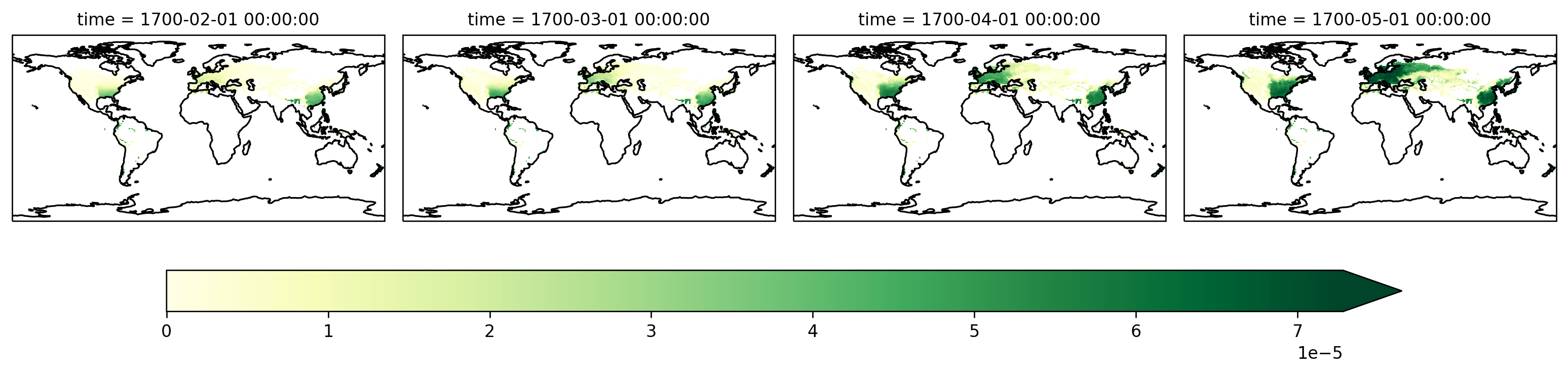
Now visualize that DataArray
fg = sparse_gpp_da.isel(vegtype=1).plot(
    col="time",
    robust=True,
    transform=ccrs.PlateCarree(),
    subplot_kws=dict(projection=ccrs.PlateCarree()),
    cbar_kwargs=cbar_kwargs,
)
[ax.coastlines() for ax in fg.axes.flat]
[<cartopy.mpl.feature_artist.FeatureArtist at 0x2ae53eaa7220>,
 <cartopy.mpl.feature_artist.FeatureArtist at 0x2ae53eaa77c0>,
 <cartopy.mpl.feature_artist.FeatureArtist at 0x2ae53fc79bb0>,
 <cartopy.mpl.feature_artist.FeatureArtist at 0x2ae53fd9dca0>]
Using xarray.apply_ufunc#
We extracted numpy arrays, called to_sparse and then used the returned sparse.COO array to manually create a DataArray. Now we wrap those steps using xarray.apply_ufunc. Why so?
apply_ufuncis really useful when you want to apply a function that expects and returns pure arrays (like numpy or sparse.COO) to an xarray object.We also anticipate using it’s automatic parallelization capabilities with dask.
We specify pft as the “input core dimension” since our function to_sparse expects this as the last dimension. apply_ufunc will automatically transpose inputs to make pft the last dimension. One clue that pft is the core dimension is that the smallest unit of data to_sparse can process is 1D along the pft dimension.
We start with this
xr.apply_ufunc(
    # function to apply
    to_sparse,
    # array inputs expected by to_sparse
    subset,
    vegtype,
    jxy,
    ixy,
    # other non-array arguments expected by to_sparse
    kwargs={"shape": (79, 192, 288)},
    # extra metadata info required by apply_ufunc
    input_core_dims=[["pft"], ["pft"], ["pft"], ["pft"]],
)
which fails with the following error message (trimmed)
---------------------------------------------------------------------------
ValueError                                Traceback (most recent call last)
/glade/scratch/dcherian/tmp/ipykernel_20245/3810394638.py in <module>

...

~/miniconda3/envs/dcpy/lib/python3.8/site-packages/xarray/core/computation.py in apply_variable_ufunc(func, signature, exclude_dims, dask, output_dtypes, vectorize, keep_attrs, dask_gufunc_kwargs, *args)
    756         data = as_compatible_data(data)
    757         if data.ndim != len(dims):
--> 758             raise ValueError(
    759                 "applied function returned data with unexpected "
    760                 f"number of dimensions. Received {data.ndim} dimension(s) but "

ValueError: applied function returned data with unexpected number of dimensions. Received 4 dimension(s) but expected 1 dimensions with names: ('time',)
Xarray complains because it received a 4D variable back (time, type, lat, lon) but only knows about the time dimension. We need to specify the rest using output_core_dims. The output looks right!
xr.apply_ufunc(
    # function to apply
    to_sparse,
    # array inputs expected by to_sparse
    subset,
    vegtype,
    jxy,
    ixy,
    # other non-array arguments expected by to_sparse
    kwargs={"shape": (79, 192, 288)},
    # extra metadata info required by apply_ufunc
    input_core_dims=[["pft"], ["pft"], ["pft"], ["pft"]],
    output_core_dims=[["vegtype", "lat", "lon"]],
)
<xarray.DataArray 'GPP' (time: 4, vegtype: 79, lat: 192, lon: 288)>
<COO: shape=(4, 79, 192, 288), dtype=float32, nnz=417656, fill_value=nan>
Coordinates:
  * time     (time) object 1700-02-01 00:00:00 ... 1700-05-01 00:00:00
Dimensions without coordinates: vegtype, lat, lon
Attributes:
    long_name:     gross primary production
    units:         gC/m^2/s
cell_methods: time: meanApply to entire dask DataArray#
Now we use xr.apply_ufunc to convert all of the data to sparse with to_sparse. This transformation can be applied to each block of a dask array independently, so we can use dask="parallelized" to automatically parallelize the operation (using something like dask.array.map_blocks underneath).
Dask will also need us to provide the sizes for these new dimensions. We do that by providing output_sizes in dask_gufunc_kwargs
xr.apply_ufunc(
    # function to apply
    to_sparse,
    # array inputs expected by to_sparse
    data.GPP,
    vegtype,
    jxy,
    ixy,
    # other non-array arguments expected by to_sparse
    kwargs={"shape": (79, 192, 288)},
    # extra metadata info required by apply_ufunc
    input_core_dims=[["pft"], ["pft"], ["pft"], ["pft"]],
    output_core_dims=[["vegtype", "lat", "lon"]],
    dask="parallelized",
    # info needed by dask to automatically parallelize with dask.array.apply_gufunc
    dask_gufunc_kwargs=dict(
        output_sizes={"vegtype": 79, "lat": 192, "lon": 288},
    ),
)
<xarray.DataArray 'GPP' (time: 3828, vegtype: 79, lat: 192, lon: 288)>
dask.array<transpose, shape=(3828, 79, 192, 288), dtype=float32, chunksize=(100, 79, 192, 288), chunktype=numpy.ndarray>
Coordinates:
  * time     (time) object 1700-02-01 00:00:00 ... 2019-01-01 00:00:00
Dimensions without coordinates: vegtype, lat, lon
Attributes:
    long_name:     gross primary production
    units:         gC/m^2/s
cell_methods: time: meanThis looks better but notice that dask still thinks its working with numpy arrays (see Type under Chunk). We need to tell dask that the output of to_sparse is a sparse array. (dask tries to detect such things automatically but for some reason that is failing; this is potentially an xarray bug).
We do that by passing the meta parameter which is an empty array with the right array type (sparse.COO) and right dtype.
xr.apply_ufunc(
    # function to apply
    to_sparse,
    # array inputs expected by to_sparse
    data.GPP,
    vegcodes,
    jxy,
    ixy,
    # other non-array arguments expected by to_sparse
    kwargs={"shape": (79, 192, 288)},
    # extra metadata info required by apply_ufunc
    input_core_dims=[["pft"], ["pft"], ["pft"], ["pft"]],
    output_core_dims=[["vegtype", "lat", "lon"]],
    dask="parallelized",
    # info needed by dask to automatically parallelize with dask.array.apply_gufunc
    dask_gufunc_kwargs=dict(
        meta=sparse.COO(np.array([], dtype=data.GPP.dtype)),
        output_sizes={"vegtype": 79, "lat": 192, "lon": 288},
    ),
)
<xarray.DataArray 'GPP' (time: 3828, vegtype: 79, lat: 192, lon: 288)>
dask.array<transpose, shape=(3828, 79, 192, 288), dtype=float32, chunksize=(100, 79, 192, 288), chunktype=sparse.COO>
Coordinates:
  * time     (time) object 1700-02-01 00:00:00 ... 2019-01-01 00:00:00
Dimensions without coordinates: vegtype, lat, lon
Attributes:
    long_name:     gross primary production
    units:         gC/m^2/s
cell_methods: time: mean👆🏾 This looks right!
Putting it all together#
Here’s a generalized function that wraps up all the steps in the previous section
Takes a Dataset like
dataas inputExtracts all variables with the
"pft"dimensionConverts to sparse arrays detecting appropriate dimension sizes
Returns a new Dataset with only
pftvariables as sparse arrays
pfts = convert_pft_variables_to_sparse(data, pftnames)
pfts
<xarray.Dataset>
Dimensions:             (lat: 192, lon: 288, vegtype: 79, time: 3828)
Coordinates:
  * lat                 (lat) float64 -90.0 -89.06 -88.12 ... 88.12 89.06 90.0
  * lon                 (lon) float64 0.0 1.25 2.5 3.75 ... 356.2 357.5 358.8
  * time                (time) object 1700-02-01 00:00:00 ... 2019-01-01 00:0...
  * vegtype             (vegtype) |S40 b'not_vegetated                       ...
Data variables: (12/15)
    pfts1d_lon          (vegtype, lat, lon) float64 dask.array<chunksize=(79, 192, 288), meta=np.ndarray>
    pfts1d_lat          (vegtype, lat, lon) float64 dask.array<chunksize=(79, 192, 288), meta=np.ndarray>
    pfts1d_ixy          (vegtype, lat, lon) float64 <COO: nnz=104414, fill_value=nan>
    pfts1d_jxy          (vegtype, lat, lon) float64 <COO: nnz=104414, fill_value=nan>
    pfts1d_gi           (vegtype, lat, lon) float64 dask.array<chunksize=(79, 192, 288), meta=np.ndarray>
    pfts1d_li           (vegtype, lat, lon) float64 dask.array<chunksize=(79, 192, 288), meta=np.ndarray>
    ...                  ...
    pfts1d_wtcol        (vegtype, lat, lon) float64 dask.array<chunksize=(79, 192, 288), meta=np.ndarray>
    pfts1d_itype_veg    (vegtype, lat, lon) float64 <COO: nnz=104414, fill_value=nan>
    pfts1d_itype_col    (vegtype, lat, lon) float64 dask.array<chunksize=(79, 192, 288), meta=np.ndarray>
    pfts1d_itype_lunit  (vegtype, lat, lon) float64 dask.array<chunksize=(79, 192, 288), meta=np.ndarray>
    pfts1d_active       (vegtype, lat, lon) float64 dask.array<chunksize=(79, 192, 288), meta=np.ndarray>
    GPP                 (time, vegtype, lat, lon) float32 dask.array<chunksize=(100, 79, 192, 288), meta=sparse.COO>
Attributes: (12/102)
    title:                                     CLM History file information
    comment:                                   NOTE: None of the variables ar...
    Conventions:                               CF-1.0
    history:                                   created on 09/27/19 16:25:57
    source:                                    Community Terrestrial Systems ...
    hostname:                                  cheyenne
    ...                                        ...
    cft_irrigated_tropical_corn:               62
    cft_tropical_soybean:                      63
    cft_irrigated_tropical_soybean:            64
    time_period_freq:                          month_1
    Time_constant_3Dvars_filename:             ./TRENDY2019_S0_constant_v2.cl...
Time_constant_3Dvars: ZSOI:DZSOI:WATSAT:SUCSAT:BSW:H...Make a test plot#
And here’s the plot we started out with
ax = setup_axes()
pfts.GPP.isel(vegtype=1, time=3606).plot(robust=True, ax=ax, cbar_kwargs=cbar_kwargs)
<cartopy.mpl.geocollection.GeoQuadMesh at 0x2ae55c00f850>
Summary#
We first developed a function
to_sparsethat took as input 1D or 2D compressed NumPy arrays and converted them tosparse.COOarrays.We then used
apply_ufuncto applyto_sparseto xarray inputs, and receive an xarray object in return.We automatically parallelized applying
to_sparseto every dask block by specifyingdask="parallelized"in theapply_ufunccall.Finally we wrote a function
convert_pfts_to_sparsethat takes an xarray Dataset as input, converts the dense 2D NumPy arrays read from disk to a 4D sparse array, and returns back a new Dataset
Question#
Are there places where sparse arrays could help in your analysis?
Start a thread on Zulip!
CF conventions for representing sparse data arrays exist: for example “compression by gathering”.
If the model output satisfied these conventions, we could write “encoder” and “decoder” functions that convert these arrays to sparse arrays (or back) in the
open_dataset/to_netcdf/to_zarrfunctions. See here for a prototype.Is anyone interested in pursuing this?